In this post we’ll be looking at compute shaders, profiling tools and failed experiments to improve performance. This is my journey learning compute shaders first through WebGPU and then Vulkan. My goal was to implement Conway’s Game Of Life algorithm in a brute force manner and to make it run as fast as possible on the GPU .

This will not be a tutorial on how to setup compute shaders. The easiest way to get started today is probably with WebGPU and this tutorial does a pretty good job at getting you through it. Once you’re familiar with the API, this example does everything you need to setup a proper Game Of Life.

Brute Force Algorithm

Conway’s Game Of Life is a cellular automaton with very simple rules. A cell lives or dies depending solely on how many of its neighbours are alive or dead. In our case, we’ll be running the simulation in a 2D grid which means a cell has 8 neighbours. The rules are as follows:

• A dead cell comes back to life or gets born if exactly 3 of its neighbours are alive.
• A living cell remains alive only if it has 2 or 3 neighbours alive.

Let’s look at a very straight forward way to implement this. Our simulation data from the previous simulation step is stored in a 1D array called srcGrid.state and the result should be stored in another 1D array called dstGrid.state. In those arrays, a dead cell is represented by 0 and a living cell is represented by 1. For now we’ll consider that somehow the GPU executes 1 thread per cell and that the variable currentCellIndex points to the right address in both srcGrid and dstGrid.

For simplicity, the grid is always square. The coordinate system uses x and y with the origin being (x : 0, y : 0) in the top left corner. I’m storing rows one after another in the 1D array.

If the grid is of size 2x2, the cells are stored in this order in the 1D array:

[ (x : 0, y : 0), (x : 1, y : 0), (x : 0, y : 1), (x : 1, y : 1) ]

The conversions to go from 1D to 2D and vice versa are as follows:

uvec2 coordinates2D = uvec2( index1D % GRID_SIZE, index1D / GRID_SIZE);
uint index1D = coordinates2D.x + coordinates2D.y * GRID_SIZE;

One last thing that might be surprising in the code below is that the simulation wraps itself around the edges. For example if a cell is on the right edge of the grid, its right neighbour is on the left edge of the grid. It’s not very important but it explains the following line:

coords = (coords + sampleXYOffsets[i] + GRID_SIZE) % GRID_SIZE;

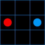
Let’s take our previous example on a 3x3 grid. The cell of coordinates (2, 1) is at the right edge of the grid. The sampleXYOffsets array contains the value (1, 0) for its right neighbour. Now if we apply the formula we get ( (2, 1) + (1, 0) + (3, 3) ) % (3, 3) = (6, 4) % (3, 3) = (0, 1). This is the cell at the left edge of the grid on the same row, as expected. In the image, the red dot cell is the ‘right neighbour’ of the blue dot cell.

Hopefully you have now all the elements in your hands to understand the main part of our first version of this compute shader.

layout(std430, set = 0, binding = 0) buffer SrcGrid
{
    uint state[CELLS_COUNT];
} srcGrid;

layout(std430, set = 0, binding = 1) buffer DstGrid
{
    uint state[CELLS_COUNT];
} dstGrid;

const ivec2 sampleXYOffsets[] =
{
    ivec2(-1, -1),   ivec2(0, -1),  ivec2(1, -1),
    ivec2(-1,  0),                  ivec2(1,  0),
    ivec2(-1,  1),   ivec2(0,  1),  ivec2(1,  1),
};

// We'll get back to this later, the point is currentCellIndex exists
SOME_MAGIC currentCellIndex;

void main()
{
    uint aliveNeighbors = 0;
    // Convert storage buffer id into grid coordinates (x, y)
    const uvec2 currentCoords = uvec2( currentCellIndex % GRID_SIZE, currentCellIndex / GRID_SIZE);
    for( uint i = 0; i < 8; i++ )
    {
        uvec2 coords = currentCoords;
        // Bring everything above 0 to be able to use the modulo operator
        coords = (coords + sampleXYOffsets[i] + GRID_SIZE) % GRID_SIZE;
        // Convert grid coordinates (x, y) into storage buffer index
        uint neighborIndex = coords.x + coords.y * GRID_SIZE;
        aliveNeighbors += srcGrid.state[neighborIndex];
    }

    uint currentCellState = srcGrid.state[currentCellIndex];
    bool isCellAlive = currentCellState > 0;

    // Dead cell comes back to life
    if( !isCellAlive && aliveNeighbors == 3 )
    {
        dstGrid.state[currentCellIndex] = 1;
        return;
    }

    // Alive cell dies
    if( isCellAlive && ( aliveNeighbors < 2 || aliveNeighbors > 3 ) )
    {
        dstGrid.state[currentCellIndex] = 0;
        return;
    }

    // Do not forget to copy the data to the new buffer even if nothing changed
    dstGrid.state[currentCellIndex] = currentCellState;
}

Dispatch and threadgroup size

In the previous section we assumed that the GPU somehow managed to map 1 thread to 1 cell and to provide us with the index of that cell in our 1D arrays. It’s actually up to the programmer to define how this mapping happens. The first thing we need to understand is that one cannot request the GPU to allocate a single thread. The only interface we get on the CPU is a threadgroup. As the name suggests, it is a group of N threads.

Software interface

Allocating threadgroups on the GPU is usually done by a variant of the dispatch command on the CPU. This command expects 3 arguments, for the x, y and z size of the threadgroup. That’s right, one can allocate threadgroups in a 1D, 2D or even 3D fashion. The total number of threadgroups dispatched is the product of x, y and z. For example, to dispatch 4 threads groups, one can either call dispatch(4, 1, 1) or dispatch(2, 2, 1). Those two commands allocate exactly the same number of threads on the GPU, the only difference is the addressing scheme we’ll talk about in a minute.

To decide how many threadgroups we want to allocate we need to know how many threads are allocated per group. Now this is where things can get confusing. Remember when I said a threadgroup is a group of N threads ? Well it’s actually a group of x * y * z threads. That’s right, one can allocate threads within a group in a 1D, 2D or even 3D fashion. Again, it doesn’t really matter what you choose for x, y and z as long as the product of the three matches your target N threads. It will however impact the addressing scheme I mentioned earlier and probably cache performance. This number is set with the local_size attribute in the shader.

If you’re like me, at this point you’re pretty confused about this whole mess. ( Especially if you’ve tried to visualize dispatching 3D threadgroups in 3D ) If it helps, think 1D only for now. We need to dispatch A groups of B threads for a total of A * B threads.

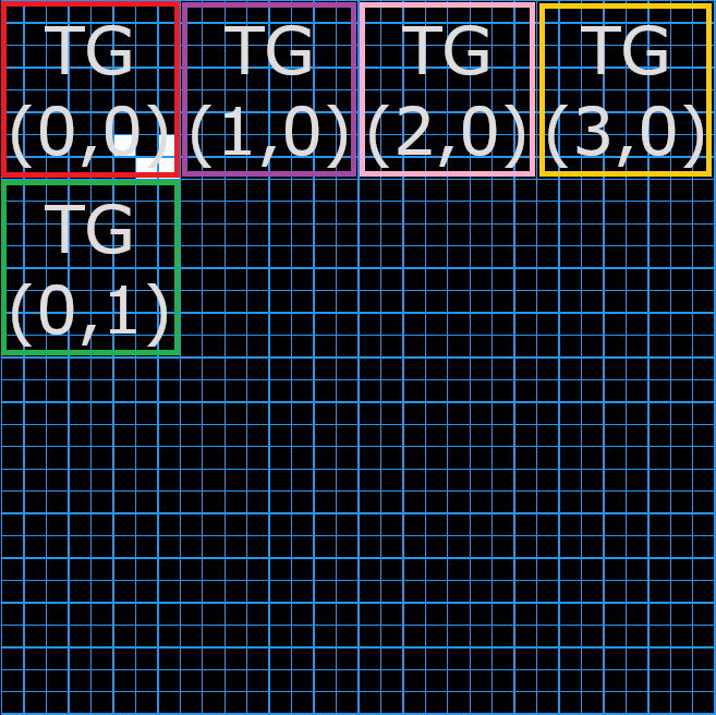
It can also help to think in 2D especially since we’re dealing with a grid. Let’s first visualize a 2D threadgroup, it’s a big patch of x by y cells on the grid. It represents N = x * y cells. Now we know that our entire grid is made of GRID_SIZE by GRID_SIZE cells. To launch a thread per cell we need to allocate enough groups of N threads to reach GRID_SIZE * GRID_SIZE threads.

Let’s take a simple example of a threadgroup of size 8 by 8 and a grid of size 32 by 32. We would need to allocate 4 groups on the x axis and 4 groups on the y axis for a total of 4 * 4 = 16 groups to cover the entire grid. Remember one group contains 8 * 8 = 64 threads, that makes a total of 64 * 16 = 1024 threads for the entire grid. We can now check our math and see that our grid of size 32 by 32 indeed needs 32 * 32 = 1024 treads.

It is entirely possible to mix and match all those dimensions to create crazy addressing schemes. One could dispatch(x, 1, z) with local_size (1, y, 1) if one were so inclined. I will deny ever putting you up to this.

A peak into the hardware

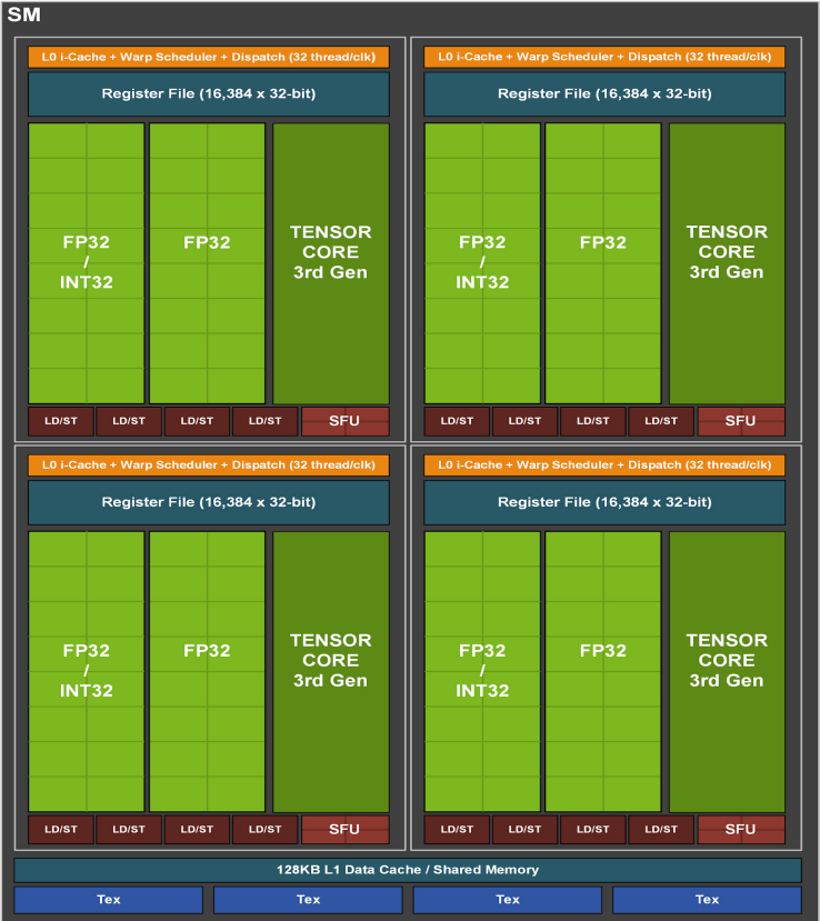
In my project, I wanted to understand this more deeply so I implemented presets which cover dispatch in 1D and 2D with local_size in 1D and 2D as well. This was very useful to realize that a threadgroup must contain a certain number of threads in order not to waste physical resources. This is due to the nature of GPUs, they issue commands in batches of fixed size. For Nvidia a batch of threads is called a warp and is 32 wide while AMD calls this a wavefront and is 64 wide. At the hardware level, theses batches are executed on Simple Instruction Multiple Data ( SIMD ) units. These SIMD units have each a wavefront scheduler and are part of a biger structure called a Compute Unit ( CU ) in AMD terminology and Streaming Multiprocessor for Nvidia. It seems both manufacturers decided to pack 4 SIMD units within a Compute Unit.

Now that we have all that in mind, let’s say we decide to create a threadgroup of 16 threads. If we try to run this on an Nvidia GPU, it will issue a warp of 32 threads and mask out the execution of half the threads. On an AMD machine it’s even worse, we would be wasting 75% of the threads per SIMD unit! This is far from being optimal and unless you have a very good reason you should not create threadgroups of less than 64 threads.

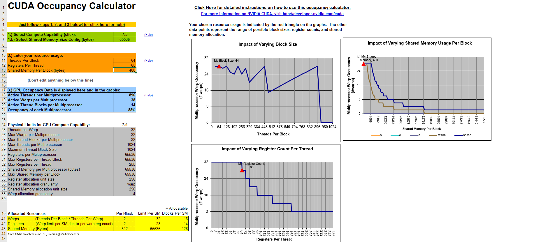
A SIMD unit is also able to schedule multiple wavefronts at the same time. It doesn’t mean that they all execute at the same time but it means that they will all execute on this specific SIMD unit. However, if a wavefront A is waiting for something, like a texture read, the SIMD scheduler can decide to replace it with another scheduled wavefront B and to resume wavefront A later when it’s ready. This is very useful to hide latency. The less clock cycles the SIMD unit is waiting for something, the more efficient it is. This metric is called occupancy. It might be a good solution then to schedule as many wavefronts per SIMD as you can to hide latency and improve occupancy. While this is true nothing is ever that simple. First there seems to be a hard limit per SIMD unit ( 10 on AMD GCN, not disclosed by Nvidia as far as I know ) and second we are also limited by the Compute Unit’s shared hardware.

The two main limiters in a Compute Unit are the VGPR ( Vector General Purpose Register ) and Shared Memory. It is important to understand that a threadgroup cannot be split across multiple Compute Units and that a wavefront can only be scheduled on a single SIMD unit. Moreover, for a wavewront to be scheduled on a SIMD unit, it needs to reserve its hardware resources within the Compute Unit first. This means that all hardware resources needed to execute all of the wavefronts of a single threadgroup must be available in a single Compute Unit. Then and only then can all the wavefronts of that threadgroup be scheduled on the different SIMD units of that Compute Unit. This goes for both VGPR and Shared Memory. To be clear, if a Compute Unit can only accept a threadgroup and a half because of register or shared memory pressure, it will only take a single threadgroup’s workload and the potential maximum occupancy of its SIMD units might get reduced.

Again, you have to run the numbers to understand potential occupancy, it might be ok to have a single threadgroup assigned if it can be split into a lot of wavefronts. That being said, the maximum size of a threadgroup is 1024 and an architecture like GCN is able handle 2 of those maximum, so it’s probably suboptimal. On top of that, the more granularity we give the scheduler, the better it can do its job.

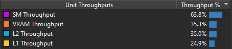
Getting back to our specific example, we can try different combinations on our computer and see which suits our GPU best. Here are a few examples on my RTX 2070 for a grid of 20000x20000. First let’s see what happens with threadgroups of size 64. The “Throughput %” metric tells us how close we are to saturating the hardware. If we reach 100%, it means that this part of the hardware cannot execute more operations. However, that doesn’t mean that we use it in an optimal way.

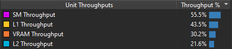
Now the same thing but with threadgroups of size 256.

In my case it appears that dispatching in 1D to a 1D local_size yields the best results. A threadgroup of size 64 or 256 doesn’t seem to have too much impact in that configuration. On the other hand, in a 2D / 2D configuration a threadgroup size of 16 x 16 is clearly faster. Unfortunately, it’s quite hard to know why for sure. Since the way threadgroups are dispatched directly impacts the order in which the cells of my simulation are treated it may also impact cache locality. There’s even a blog post called Optimizing Compute Shaders for L2 Locality using Thread-Group ID Swizzling about this but it’s not super relevant to our program.

First optimization - Nsight Driven

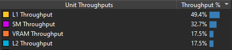
Ok so now we know what the software interface is, we have some idea of what the hardware constraints are and our first version of the shader works. It is very straight forward - read all the neighbors, count the living cells and then overwrite the result with whatever state we got. What does Nsight say about this? This is what it looks like in steady state for a 20k by 20k grid, dispatch in 1D using 1D threadgroup size of 64 on my RTX 2070.

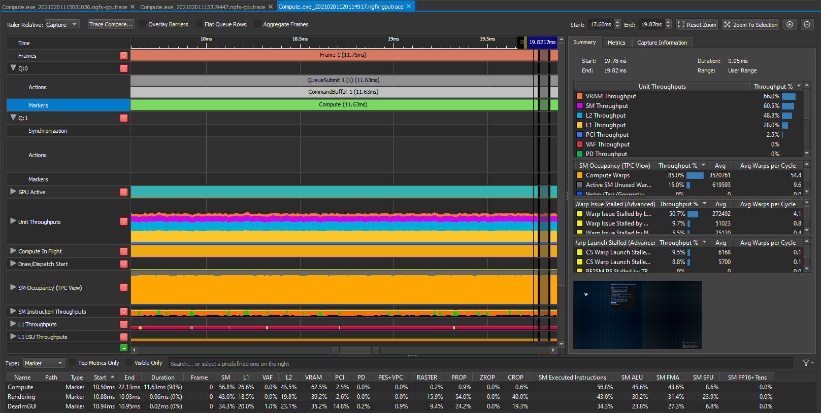
Meh, it looks ok to me at 11.5ms, I don’t know, maybe? I had no clue really so I watched a few talks from Nvidia on how to use the tool and make sense of the data it provides. They mostly advertise the P3 method Peak Performance Percentage which relies on multiple metrics. This blog post is a bit outdated and relies on the Frame Profiler part of Nsight but it still provides a lot of insight on how the tool works.

We’ll be using the latest and greatest part of Nsight called GPU trace instead ( available with Turing ) because it suits async compute workloads better. There is yet another Nvidia blog post about it here. If you read the old blog post, you can replace SOL by throughput which is their newest terminology but it exactly the same thing.

Ok so following the method we’ll want to investigate the top throughput units first. On the right part of the screenshot, you can see that the VRAM is at 66%. According to the method, this means we’re either limited by the latency of the VRAM or we’re giving it too much work. The third top limiter is L2 though at a low 48% so let’s suppose we’re latency limited for now and investigate that path. This is also convenient because that’s exactly what the second blog post I linked is investigating as well :p.

Since our VRAM is our top limiter, we might want to investigate how it is accessed and if we can do better. Here is what the blog post has to say about this.

On all NVIDIA GPUs after at least Fermi, all VRAM traffic goes through the L2 cache, so we can use L2 metrics to understand what requests are made to the VRAM.

This makes sense, we have a low throughput for L2 too. So Nsight lets you see through the metrics tab what unit accessed the L2 cache. The blog post mentions searching for srcunit which doesn’t work anymore but looking for L2 will do the trick. Here is what we get for that search.

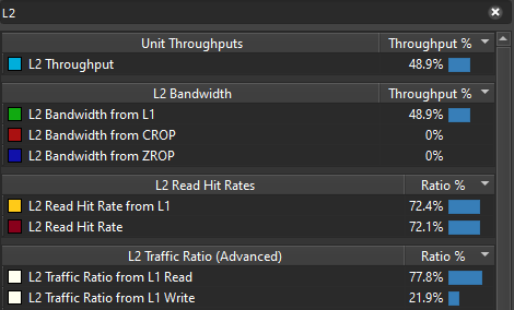
That’s interesting, if we look at the L2 Traffic Ratio 20% of overall traffic is dedicated to writing while 80% is dedicated to reading. It makes sense because for each cell, we have to read 9 cells and only write to one. However, this sounds like a lot of writing. What if my board is really sparse? I’m usually testing with a single planner moving through the grid, we can make this faster for this use case.

The writes we want to get it rid of are the ones that copy data from one SSBO to another when the data didn’t change. Basically, we want to get rid of the last line of the shader when the data didn’t change.

// Do not forget to copy the data to the new buffer even if nothing changed
dstGrid.state[currentCellIndex] = currentCellState;  

If nothing changed, let’s not make useless writes. With very little changes to the code, we can register which cells changed in the last rotation in order to avoid redundant copies. Instead of storing 1 for a cell that is alive and 0 for a dead cell, we’ll store 3 for a cell that is alive and was just updated and 2 for a dead cell that was just updated. This allows us to easily check if the cell is alive or not with a simple cellState % 2 and barely changes our shader.

uint currentCellState = srcGrid.state[currentCellIndex];
bool isCellAlive = currentCellState % 2 == 1;

// Dead cell comes back to life
if( !isCellAlive && aliveNeighbors == 3 )
{
    dstGrid.state[currentCellIndex] = 3;
    return;
}

// Alive cell dies
if( isCellAlive && ( aliveNeighbors < 2 || aliveNeighbors > 3 ) )
{
    dstGrid.state[currentCellIndex] = 2;
    return;
}   

And now we have the info we need to ditch that last write. If none of the 2 above ifs are triggered, we enter the part of the code that does a stupid copy. But now, we can check the value of the current state and figure out whether it was updated during the last iteration. If its value is greater than 1 ( 2 or 3 ), than yes it was updated in the last rotation and we need to update the dst SSBO. We also want to flag this cell as up to date and for that, we’ll use our old state code: 0 for dead and 1 for alive. This doesn’t break our previous test to check if a cell is alive or dead.

// If this cell was previously modified, update it. Otherwise it's already up to date.
if( currentCellState > 1 )
{
    dstGrid.state[currentCellIndex] = currentCellState - 2;
}    

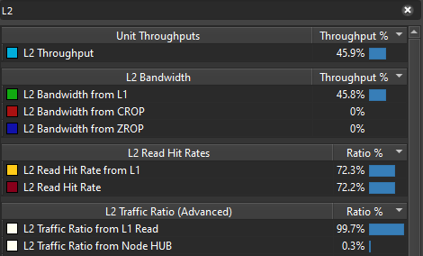
So what does Nsight have to say about this modification?

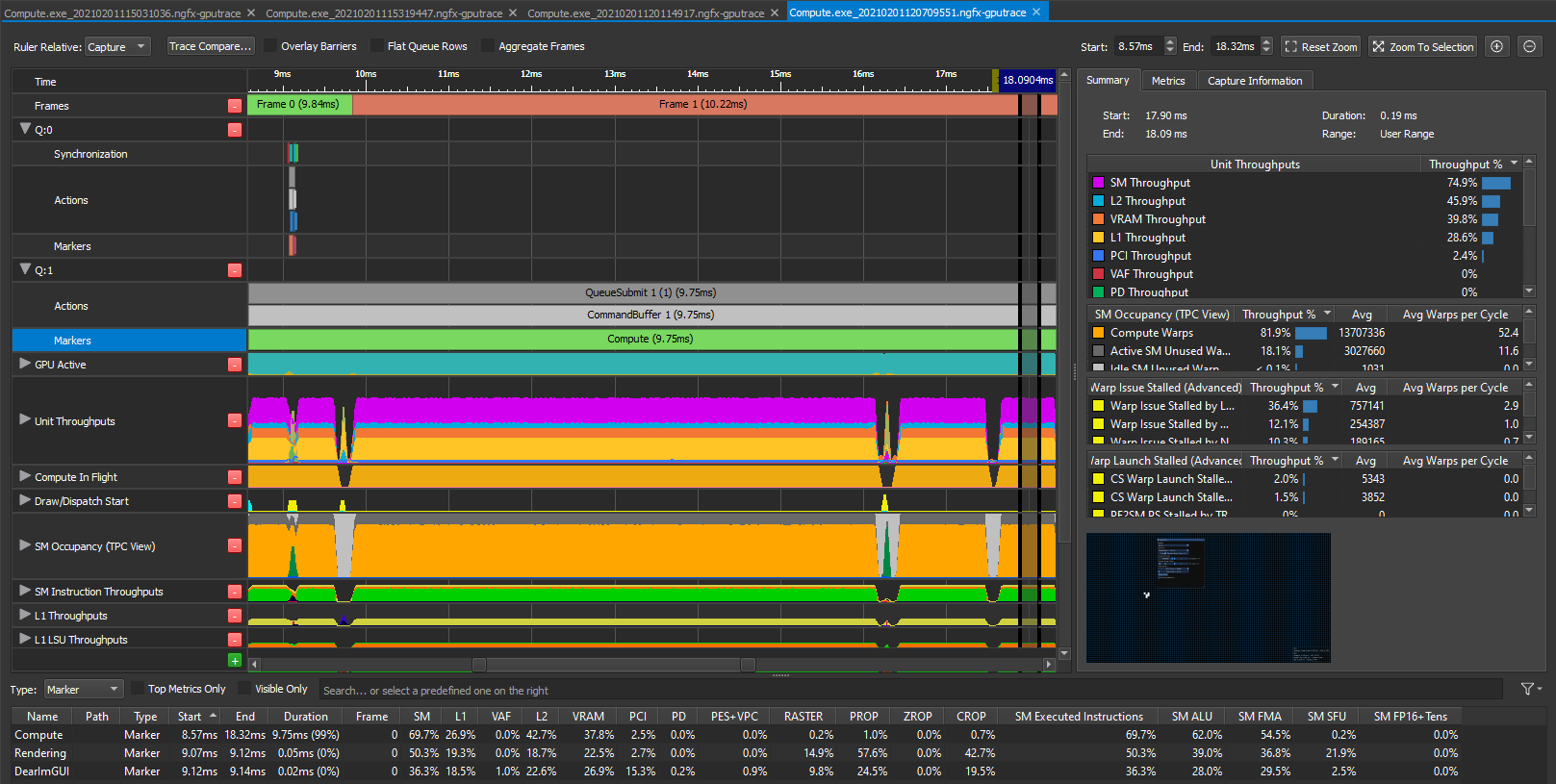
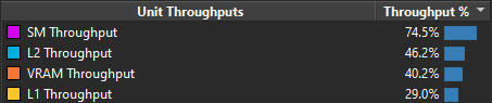
Whoohoo, we almost shaved of 2ms it’s about 20% faster! Go us! If we look at our top throughput units, SM is now at 75% and VRAM and L2 are kept in check way below at around 40-45%. That’s a great win! And without any surprises, if we look at our L2 traffic origin, we can see that 99.7% of our L2 traffic comes L1TEX Reads!

That’s a nice win, we profiled the app, found a bottleneck with Nsight, fixed it with minimal code change and it’s actually faster! As a reminder, this optimization is mostly valid for sparse grids. I have tried filling the grid with random data and the compute pass takes about 13.5ms to complete. This is worse than our original solution though, so to be used with caution.

Coming Soon

In the next blog post I will be investigating more ways to optimize this shader further.

One idea that succeeded was to make each thread read multiple cells from the SSBO, store them in registers and then process them. This used to be way slower on my RTX 2070 until I recently updated my graphics drivers and Vulkan version. I’m not sure which did the trick but it is now faster than the brute force version. The size of the island is limited by register pressure though.

I have also tried the previous technique but with shared memory, I’ve tried to use uint8 data instead of full blown floats, I’ve tried to use subgroup ballot operations and even swizzling tiles without any luck. I’ll go over those failed attempts as well.

I’ll hopefully see you for part two, in the meantime here is a bonus thread about a weird bug I encountered! https://twitter.com/frguthmann/status/1299002817412321281?s=20